Explore a GBIF dataset – Elasticsearch/Kibana

In this post I will explain how to sync a PostgreSQL table to an Elasticsearch index using Debezium. This is a follow-up on my previous post. In that post I explained how to load a GBIF dataset into a PostgreSQL database.

Debezium’s PostgreSQL connector captures row-level changes in the schemas of a PostgreSQL database. This technique is called Change Data Capture (CDC) and can be used to sync a database table to (in this case) Elasticsearch. CDC makes it possible to move heavy search workloads away from the database.

In this example I’m going to explain how to sync a table named explore.gbif to an Elasticsearch index named db1.explore.gbif, using the following components:

Download this docker-compose project to try this setup on your local computer using Docker. After starting the containers the dataset will be downloaded and inserted into a PostgreSQL table.

When all containers are up, run the sync_to_elasticsearch.sh script. This script will do the following:

• Create an index and field mappings
• Setup the PostgreSQL source connector
• Setup the Elasticsearch sink connector

There are three fields that need a mapping, gbifid, eventdate and location. The location field is used to plot locations on a world map in Kibana:

{
  "settings": {
    "number_of_shards": 1
  },
  "mappings": {
    "properties": {
      "gbifid": {
        "type": "long"
      },
      "eventdate": {
        "type": "date"
      },
      "location": {
        "type": "geo_point"
      }
    }
  }
}

The psql connector is used to create the connection between kafka and the database. Notice the column.blacklist setting to exclude the PostGIS geometry and tsv columns.

{
  "name": "psql_connector",
  "config": {
        "connector.class": "io.debezium.connector.postgresql.PostgresConnector",
        "tasks.max": "1",
        "database.hostname": "postgres",
        "database.port": "5432",
        "database.user": "postgres",
        "database.password": "postgres",
        "database.dbname": "db1",
        "database.server.name": "db1",
        "database.whitelist": "db1",
        "heartbeat.interval.ms": "1000",
        "table.whitelist": "explore.gbif",
        "column.blacklist":"explore.gbif\\.(geom|tsv).*",
        "database.history.kafka.bootstrap.servers": "kafka:9092",
        "plugin.name": "pgoutput"
  }
}

The Elasticsearch connector is used to connect kafka to the Elasticsearch instance. The transforms.key.field is set to gbifid, the primary key in the table.

{
  "name": "es_connector",
  "config": {
    "connector.class": "io.confluent.connect.elasticsearch.ElasticsearchSinkConnector",
    "tasks.max": "1",
    "topics": "db1.explore.gbif",
    "connection.url": "http://elasticsearch:9200",
    "transforms": "unwrap,key",
    "transforms.unwrap.type": "io.debezium.transforms.UnwrapFromEnvelope",
    "transforms.unwrap.drop.tombstones": "false",
    "transforms.unwrap.drop.deletes": "false",
    "transforms.key.type": "org.apache.kafka.connect.transforms.ExtractField$Key",
    "transforms.key.field": "gbifid",
    "key.ignore": "false",
    "type.name": "_doc",
    "behavior.on.null.values": "delete"
  }
}

Using the docker-compose logs command to see that the table is being synced to the Elasticsearch index:

Use the following command to see when the sync is finished:

docker-compose logs -f connect

docker-compose logs connect | grep 'Finished exporting'

A log line should like this should show after a couple of minutes:

Finished exporting 287671 records for table 'explore.gbif'; total duration '00:01:41.021'   [io.debezium.relational.RelationalSnapshotChangeEventSource]

Now let’s check if all records are synced to Elasticsearch. Query the number of records in the Elasticsearch index:

curl http://localhost:9200/db1.explore.gbif/_count

{
  "count": 287671,
  "_shards": {
    "total": 1,
    "successful": 1,
    "skipped": 0,
    "failed": 0
  }
}

Query the number of records in the table. Both queries show the same number, this confirms that all records are correctly synced:

docker-compose exec postgres bash -c 'psql -U $POSTGRES_USER $POSTGRES_DB -c "SELECT COUNT(*) FROM explore.gbif"'

 count
--------
 287671
(1 row)

The next step is to load a Kibana dashboard using the script called load_kibana_dashboard.sh. Run this script. The output of this script should look like this:

Load Kibana dashboard                                           
{"success":true,"successCount":7}

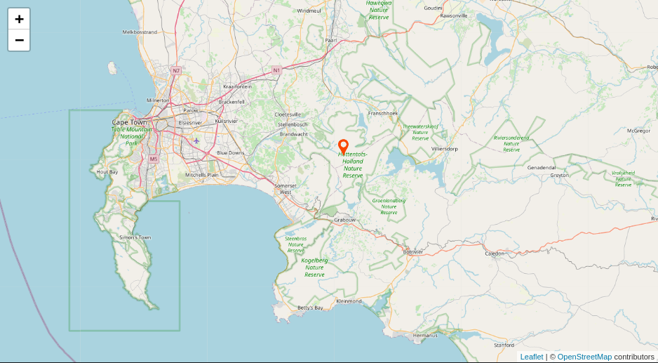
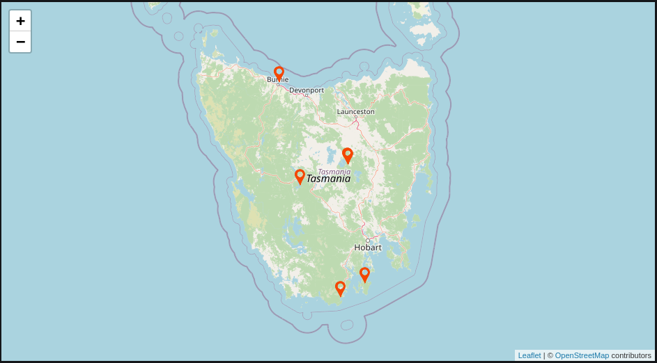
Now browse to http://localhost:5601/app/kibana#/dashboards. Click on the dashboard called Explore a GBIF dataset.

Compare the map in Kibana (above) with the map in Grafana (below). As you can see the data is identical.

Record with gbifid 2434193680 in the database:

SELECT * FROM explore.gbif WHERE gbifid IN (2434193680):

gbifid               | 2434193680
eventdate            | 1781-01-01 00:00:00+00
year                 | 1781
month                | 1
day                  | 1
catalognumber        | RMNH.AVES.87036
occurrenceid         | https://data.biodiversitydata.nl/naturalis/specimen/RMNH.AVES.87036
recordedby           | Levaillant F.
sex                  | FEMALE
lifestage            | JUVENILE
preparations         | mounted skin
locality             |
stateprovince        | Cape of Good Hope
countrycode          | ZA
higherclassification | Phalacrocoracidae
kingdom              | Animalia
phylum               | Chordata
class                | Aves
order                | Suliformes
family               | Anhingidae
genus                | Anhinga
specificepithet      | melanogaster
species              | Anhinga rufa
genericname          | Anhinga
scientificname       | Anhinga melanogaster rufa (Daudin, 1802)
decimallatitude      | -34.0083
decimallongitude     | 19.0083
geom                 | 0101000020E61000008A8EE4F21F023340454772F90F0141C0
location             | -34.0083,19.0083

The same record in the Elasticsearch index:

GET /db1.explore.gbif/_search?q=gbifid:2434193680

{
  "took" : 22,
  "timed_out" : false,
  "_shards" : {
    "total" : 1,
    "successful" : 1,
    "skipped" : 0,
    "failed" : 0
  },
  "hits" : {
    "total" : {
      "value" : 1,
      "relation" : "eq"
    },
    "max_score" : 1.0,
    "hits" : [
      {
        "_index" : "db1.explore.gbif",
        "_type" : "_doc",
        "_id" : "2434193680",
        "_score" : 1.0,
        "_source" : {
          "gbifid" : 2434193680,
          "eventdate" : "1781-01-01T00:00:00Z",
          "year" : 1781,
          "month" : 1,
          "day" : 1,
          "catalognumber" : "RMNH.AVES.87036",
          "occurrenceid" : "https://data.biodiversitydata.nl/naturalis/specimen/RMNH.AVES.87036",
          "recordedby" : "Levaillant F.",
          "sex" : "FEMALE",
          "lifestage" : "JUVENILE",
          "preparations" : "mounted skin",
          "locality" : null,
          "stateprovince" : "Cape of Good Hope",
          "countrycode" : "ZA",
          "higherclassification" : "Phalacrocoracidae",
          "kingdom" : "Animalia",
          "phylum" : "Chordata",
          "class" : "Aves",
          "order" : "Suliformes",
          "family" : "Anhingidae",
          "genus" : "Anhinga",
          "specificepithet" : "melanogaster",
          "species" : "Anhinga rufa",
          "genericname" : "Anhinga",
          "scientificname" : "Anhinga melanogaster rufa (Daudin, 1802)",
          "decimallatitude" : -34.0083,
          "decimallongitude" : 19.0083,
          "location" : "-34.0083,19.0083"
        }
      }
    ]
  }
}

Happy exploring!

Explore a GBIF dataset – PostgreSQL/Grafana

In this article I am going to explain how to setup an open-source visualization stack to explore a GBIF dataset using PostgreSQL and Grafana. The Global Biodiversity Information Facility (GBIF) is an international organisation that focuses on making scientific data on biodiversity available via the Internet using web services. The dataset that I use in this demo can be found here.

Dataset characteristics:

• 287.671 records
• 249 columns
• 51% with coordinates

Download this docker-compose project to try this setup on your local computer using Docker. After starting the containers the dataset will be downloaded into the PostgreSQL container and the queries shown below will be applied. The end result is a Grafana dashboard that uses PostgreSQL as backend. This is a screenshot of the dashboard that shows specimens found in Indonesia between 1800 and 1855:

Create queries and tables

Download and unpack the dataset using the following commands:

wget https://api.gbif.org/v1/occurrence/download/request/0107080-200613084148143.zip
unzip 0107080-200613084148143.zip

The file containing the data we are interested in is named occurrence.txt.

Convert column names in header to lowercase:

awk 'NR==1{$0=tolower($0)} 1' occurrence.txt > occurrence.tsv

Export the first 10 lines as reference records:

head -n 10 occurrence.tsv > occurrence_reference.tsv

Remove header line:

tail -n +2 occurrence.tsv > gbif_raw.tsv

Use csvkit to create a CREATE TABLE statement. Copy the resulting query and execute it on your PostgreSQL database instance:

csvsql --tabs --dialect postgresql --no-constraints --db-schema explore --tables gbif_raw occurrence_reference.tsv > create_table.sql

Set the table to UNLOGGED to prevent creating excessive WAL files when running UPDATE statements. Run on your PostgreSQL instance:

ALTER TABLE explore.gbif_raw SET UNLOGGED;

Create SQL code to set all columns to datatype ‘text’. Copy the resulting queries and execute them on your PostgreSQL database instance:

SELECT 'ALTER TABLE ' || table_schema || '.' || table_name || ' ALTER COLUMN "' || column_name || '" TYPE text;' FROM information_schema.columns WHERE table_name = 'gbif_raw' AND table_schema = 'explore';

Create a schema and import the data. Run on your PostgreSQL instance:

CREATE SCHEMA explore;
COPY explore.gbif_raw FROM '/tmp/gbif_raw.tsv' DELIMITER E'\t';

Create SQL code to set empty strings to null on a subset of columns. Copy the resulting queries and execute them on your PostgreSQL database instance:

SELECT 'UPDATE ' || table_schema || '.' || table_name || ' SET "' || column_name || '" = null WHERE "' || column_name || '" = '''';' FROM information_schema.columns WHERE table_name = 'gbif_raw' AND table_schema = 'explore' AND column_name IN (
 'gbifid', 
 'eventdate',
 'year',
 'month',
 'day',
 'catalognumber', 
 'occurrenceid', 
 'recordedby', 
 'sex', 
 'lifestage', 
 'preparations', 
 'locality', 
 'stateprovince', 
 'countrycode', 
 'higherclassification', 
 'kingdom', 
 'phylum', 
 'class', 
 'order', 
 'family', 
 'genus', 
 'specificepithet',
 'species',
 'genericname',
 'scientificname',
 'decimallatitude',
 'decimallongitude'
 );

Create the table and some indexes. Run on your PostgreSQL instance::

CREATE EXTENSION postgis;

CREATE TABLE explore.gbif (
 gbifid bigint PRIMARY KEY,
 eventdate timestamptz,
 year int,
 month int,
 day int,
 catalognumber text,
 occurrenceid text,
 recordedby text,
 sex text,
 lifestage text,
 preparations text,
 locality text,
 stateprovince text,
 countrycode text,
 higherclassification text,
 kingdom text,
 phylum text,
 class text,
 "order" text,
 family text,
 genus text,
 specificepithet text,
 species text,
 genericname text,
 scientificname text,
 decimallatitude float,
 decimallongitude float,
 geom geometry(POINT,4326),
 location text,
 tsv tsvector
);

CREATE INDEX ON explore.gbif USING BTREE (eventdate);
CREATE INDEX ON explore.gbif USING GIST (geom);

Create function with trigger to populate the geom column, to be able to perform postgis queries. Also create a function with a trigger to populate the location column for use in Elasticsearch. Run on your PostgreSQL instance:

CREATE OR REPLACE FUNCTION explore.update_geom() RETURNS TRIGGER AS 
 $$
   BEGIN 
     NEW.geom := ST_SetSRID(ST_Makepoint(NEW.decimallongitude,NEW.decimallatitude),4326);
     RETURN NEW;
   END;
 $$ LANGUAGE 'plpgsql';

CREATE TRIGGER update_geom BEFORE INSERT OR UPDATE ON explore.gbif FOR EACH ROW EXECUTE PROCEDURE explore.update_geom();

CREATE OR REPLACE function explore.update_location() RETURNS TRIGGER AS 
 $$
   BEGIN
     IF NEW.decimallatitude IS NOT NULL AND NEW.decimallongitude IS NOT NULL THEN
       NEW.location := concat_ws(',', NEW.decimallatitude, NEW.decimallongitude);
     END IF;
     RETURN NEW;
   END;
 $$ LANGUAGE 'plpgsql';

CREATE TRIGGER update_location BEFORE INSERT OR UPDATE ON explore.gbif FOR EACH ROW EXECUTE PROCEDURE explore.update_location();

Insert the data

Insert data into table explore.gbif from table explore.gbif_raw. Run on your PostgreSQL instance::

INSERT INTO explore.gbif (SELECT
 gbifid::bigint, 
 eventdate::timestamptz,
 year::int,
 month::int,
 day::int,
 catalognumber, 
 occurrenceid, 
 recordedby, 
 sex, 
 lifestage, 
 preparations, 
 locality, 
 stateprovince, 
 countrycode, 
 higherclassification, 
 kingdom, 
 phylum, 
 class, 
 "order", 
 family, 
 genus, 
 specificepithet,
 species,
 genericname,
 scientificname,
 decimallatitude::float,
 decimallongitude::float
 FROM explore.gbif_raw
);

Grafana

The Grafana dashboard consists of three panels, the trackmap panel, a histogram panel and a table panel that can be used to browse through the data based on time and location. I chose the trackmap panel created by the Alexandra Institute above the worldmap panel from Grafana Labs because of the map bounds functionality.

This map shows clusters of specimens found in Southern Africa using the following query:

WITH a AS (
 SELECT
 eventdate AS time,
 decimallatitude,
 decimallongitude,
 geom,
 COUNT(*) OVER() AS cnt
 FROM explore.gbif
 WHERE eventdate BETWEEN '1780-01-01T23:00:00Z' AND '2020-12-31T23:00:00Z'
 AND decimallatitude >= -45.82879925192133
 AND decimallatitude <= 45.583289756006316
 AND decimallongitude >= -248.20312500000003
 AND decimallongitude <= 248.55468750000003
 ), b AS (
 SELECT
 time,
 decimallatitude,
 decimallongitude,
 ST_ClusterKMeans(geom, LEAST(cnt::integer, 150)) OVER() AS clusters
 FROM a
 )
 SELECT
 clusters,
 COUNT(clusters) AS tooltip,
 AVG(decimallatitude) AS latitude,
 AVG(decimallongitude) AS longitude
 FROM b
 GROUP BY 1
 ORDER BY 1;

Zoom to a specific area and show the records in a table:

The two specimens shown in the tabel are the oldest in this dataset. Use the link in the occurrenceid column to check the information and see an image of these specimens, gathered by François Levaillan in 1781.

Happy exploring!

PostgreSQL 10 running in Docker

Before the end of this year PostgreSQL version 10 will be released. In this post I will explain how you can already have a quick look at this new version by running it in a Docker container.

On my Github page you can find a docker-compose file with five defined containers: an ELK stack, pgAdmin and a PostgreSQL instance. The ELK stack will be used for collecting logs from the PostgreSQL instance. I am using a host machine running Ubuntu 16.04 with Docker version 17.05.0 and Docker Compose version 1.9.0. In the Kibana dashboard, you will be able to see an overview of all the SQL statements done by a pg_restore command, and look for any errors.

First step is to download the Github repository:

git clone -b v1.0 https://github.com/rudibroekhuizen/docker-postgresplus

Move to the docker-postgresplus folder and run the following command:

docker-compose up

The containers will start. Start an interactive session to the Postgres container:

docker exec -it dockerpostgresplus_postgres_1 sh

Download Sakila example database:

wget https://s3.amazonaws.com/assets.datacamp.com/course/sql/dvdrental.zip; unzip dvdrental.zip

Create the Sakila database and import data:

su postgres
psql
psql> CREATE DATABASE sakila;
/q
pg_restore -U postgres -d sakila dvdrental.tar

Open the Kibana webinterface and import the dashboard.json file:

http://localhost:5601

Now it is possible to see what and how many statements where issued by pg_restore and how long they took:

Open the pgAdmin webinterface to browse through all tables in the Sakila database:

http://localhost:5050

Hostname, username and password are all set to “postgres”.

Trace PostgreSQL queries using logging collector

A great way to see what queries are being executed and how long they take is by enabling the logging collector on your PostgreSQL database server. The logging collector is a background process which captures log messages sent to stderr and redirects them into log files.  Make sure the following settings are set in postgresql.conf:

logging_collector = on
log_min_duration_statement = 0
log_directory = '/var/log/postgresql'
log_min_messages = WARNING
log_rotation_age = 1d
log_rotation_size = 1GB
log_line_prefix = 'start_prefix{"log_time":"%m","application_name":"%a","user_name":"%u","database_name":"%d","remote_host":"%r","process_id":"%p","command_tag":"%i","sql_state":"%e","session_id":"%c","session_line_number":"%l","virtual_transaction_id":"%v","session_id":"%c"}end_prefix log_line: '

To log only actions that took more than for example 5 ms, set the value to 5. If set to 0, all actions will be logged, to disable, set to -1.

I changed the notation of the log_line_prefix to JSON format, so that this part can be easily parsed by Logstash.

Restart the PostgreSQL to make these settings active. My test setup:

– A Drupal installation on a LAPP stack (Linux, Apache, PostgreSQL, php) with Filebeat installed to ship the logs
– An ELK stack (Elasticsearch, Logstash, Kibana) to parse the logs and make the results visible

In directory /var/log/postgres you will find *.log files with log lines that look like the following:

start_prefix{"log_time":"2017-06-09 14:09:29.141 CEST","application_name":"[unknown]","user_name":"drupal_user","database_name":"drupaldb","remote_host":"::1(49408)","process_id":"8412","command_tag":"SELECT","sql_state":"00000","session_id":"593a8ff9.20dc","session_line_number":"8","virtual_transaction_id":"2/0","session_id":"593a8ff9.20dc"}end_prefix log_line: LOG: duration: 0.501 ms statement: SELECT cid, data, created, expire, serialized, tags, checksum FROM cache_data WHERE cid IN ( 'route:/search/node:keys=foobar' ) ORDER BY cid

The actual log_line should also be parsed, to get the duration value out. The complete Logstash filter can be found on this Github page. The end result in Elasticsearch will look like this:

Now make Drupal run some queries, search for ‘helloworld’:

A search for ‘helloworld’ in Elasticsearch will show that three queries where executed, two SELECT queries and one INSERT query:

With pg_stat_activity it is possible to get (almost) the same results, but there are a few drawbacks with this approach:
– Logs can not be shown real-time, scheduled queries are needed to get the information out of the pg_stat_activity table.
– The duration of the action is not available. To see query times, you need to load the pg_stat_statements module, which requires additional shared memory.

The logging collector collects all logs, not only query logs, so you will have all logs in one place. If you haven’t seen enough log line, set log_min_messages to DEBUG5, which will show you all logs possible from your database server.

Connect to PostgreSQL database from pgAdmin4 running in Docker container using ssh tunnel

The latest version of pgAdmin, version 4, is not available in the Ubuntu repo’s. To install you need to install Python, set up an virtual environment, etc. It’s a lot easier to run pgAdmin from a Docker container. In this post I will explain how to set this up and create a secure ssh tunnel to your PostgreSQL database from the container.

Install Docker with this simple script:

sudo curl -sSL https://get.docker.com/ | sh

Start the Docker service:

sudo service docker start

Download and start the pgAdmin container:

docker run -p 5050:5050 --name pgadmin nphung/pgadmin

Now open your browser and navigate to http://127.0.0.1:5050. You should see something like this:

The safest way to connect to your database is to use ssh. You don’t need to open up any additional ports this way. Issue the following command on your local computer:

ssh -fNg -L 172.16.1.2:5432:localhost:5432 35.156.108.86

The fist IP adres and port (172.16.1.2:5432) is the IP of your local computer. In your case it will be different, use the command ip addr to look it up. The port 5432 is the port you will be connecting to.

The second IP and port is the address of your PostgreSQL database server.

Now go to your browser and right-click on Servers, Create”, Server”.

Enter a name in the General tab. Enter IP address, User name and Password and press Save:

Now right-click on the entry you just made and click Connect Server. You should now be connected to your database server.

Configure pfSense using YAML data

Configuring a pfSense firewall using the web-interface works, but it takes a lot of time. With the developer shell you can configure your device using commands. There are already some posts on this topic, this one and this one. Using the simple ruby script on my Github page it is possible to create developer shell commands using a YAML file as input. In VirtualBox it is simple to set up a testing environment. Do a clean install, and enable ssh:

Temporarily allow all traffic on the WAN interface using pfSense Developer Shell:

Example YAML file:

#master.yaml:

system:
  hostname: 'master'
  domain: 'localdomain'
  dnsserver:
    '0': '8.8.8.8'
    '1': '8.8.4.4'

Run the Ruby script:

ruby creator.rb master.yaml > master.conf

This will create a .conf file containing developer shell commands:

#master.conf:

$config['system']['hostname'] = 'master';
$config['system']['domain'] = 'localdomain';
$config['system']['dnsserver']['0'] = '8.8.8.8';
$config['system']['dnsserver']['1'] = '8.8.4.4';
write_config();
exec
exit

Apply all settings from your Linux machine using ssh:

ssh root@192.168.1.122 '/usr/local/sbin/pfSsh.php' < master.conf

Reboot, log on the webinterface and skip the welcome wizard. All settings are applied:

Analyse tshark capture in Kibana

Tshark is the terminal version of the packet capture application Wireshark. Using Tshark in combination with an ELK stack (Elasticsearch, Logstash, Kibana) it is possible to display your capture results in graphs. In this post I will explain how to capture network traffic, send it to Elasticsearch using Logstash and display graphs in Kibana. As a client I used Windows, the ELK server runs on Ubuntu.

The following command will capture network traffic for 1 minute. Once it is finished, it will run again, and so on. This will prevent memory issues with tshark and a very large .csv file. It will create a .csv file. Install Wireshark and go to C:\Program Files\Wireshark. Now run tshark:

for /L %G in (*) do tshark -a duration:60 -i 1 -t ad -lT fields -E separator=, -E quote=d -e _ws.col.Time -e _ws.col.Source -e _ws.col.Destination -e ip.src -e ip.dst -e tcp.srcport -e tcp.dstport -e _ws.col.Protocol -e ip.len -e _ws.col.Info > C:\Windows\Temp\tshark.csv

The resulting .csv file will contain lines like that look like this:

"2016-02-12 20:04:12.137523", "123.123.45.234", "192.168.1.1", "123.123.45.234", "192.168.1.1", "443", "63103", "TLSv1.2", "987", "Application Data"

On the Windows client Logstash or Filebeat needs to be installed to transport the .csv file to Elasticsearch. Filebeat is designed for this, you can install it using a Puppet module. On the ELK server Logstash will pick up the beat and apply a filter. Use the csv filter to assign the correct field names to the values in the .csv file.

filter {
   csv {
     source => "message"
     columns => [ "col.Time", "col.Source", "col.Destination", "ip.src", "ip.dst", "tcp.srcport", "tcp.dstport", "col.Protocol", "ip.len", "col.Info" ]
   }
   mutate {
     convert => [ "ip.len", "integer" ]
   }
   date {
     match => [ "col.Time", "YYYY-MM-dd HH:mm:ss.SSSSSS" ]
   }
  }

Send the results to Elasticsearch, and Kibana will show the data. Now you can start analyzing your network data:

Enjoy analyzing!

Windows metrics: part 2

There are two options to get Logstash running on your Windows machine. The first option is a manual installation. You need to download some files, install Java and copy your Logstash config file to the right folder. Another option is to let Puppet install it for you, which is faster and can be repeated easily. On github.com you can find a Puppet module to install Logstash on Windows. I have created a role module which applies the Puppet module and also installs jq and the script mentioned in part 1 of this series.

When using the Get-EventLog System command it is is possible to collect events from Windows eventviewer. In the following screenshot you can see some result in Kibana 4.

Windows metrics: part 1

So you want to know what is happening on your Windows machine? You can with Logstash!

Using Logstash you can collect and process all sorts of event logs. There are various input filters available, for both Linux and Windows. Since PowerShell version 4 it is possible to display PowerShell output in JSON format. This option makes it very easy to import PowerShell output into Logstash.

PowerShell can retrieve any fact about your Windows system, for example memory usage, disk space usage, cpu load, but also events from event viewer, account information from Active Directory, Radius logons from NPS, etc. etc. The possibilities are endless!

Lets take available memory as an example, run in PowerShell:

convertto-json @(Get-WmiObject Win32_OperatingSystem | select FreePhysicalMemory) | Out-File "C:/Windows/Temp/json_array.json" -encoding utf8

Open the file C:/Windows/Temp/json_array.json and you will see something like this:

[
    {
        "FreePhysicalMemory":  254436
    }
]

To use this as an input for Logstash, we will need to do some formatting on this output. Every new line in a textfile is a new event for Logstash. There is a great tool called jq, which can do just what we need. Again, run this in PowerShell:

cmd /c "jq -c .[] < C:/Windows/Temp/json_array.json" | Out-File -Append -NoClobber "C:/Windows/Temp/json_objects.json" -encoding utf8

Open the file C:/Windows/Temp/json_objects.json and you will see something like this:

{"FreePhysicalMemory":254436}

Everytime we run the two commands, an extra line will be added, a new event on every line. This is the sort of input we need for Logstash! In part 2 you can learn how to create the Logstash filters.

Learning Puppet for Windows Server

Earlier this year I was contacted by UK publishing house Packt Publishing about being a technical reviewer for a book called “Learning Puppet for Windows Server”. The book will be published later this month!